Inverse Kinematics

Inverse Kinematics (IK) is the process of finding the required joint angles or positions of a robot at a specific target position and orientation in space.

Usually multiple solutions are possible to solve this problem; it is possible to adopt different approaches.

If the structure is simple enough as in planar robots or 6-axis antropomorphic arms with spherical wrist (kinematic decoupling), it is possible to derive the joint angles/distances analytically.

If the structure of the robot is complex, it is possible to use some numerical methods such as Jacobian Inverse Method/PseudoInverse

In addition, it’s possible to use Neural Networks and more advanced algorithms.

Two Link Planar Arm

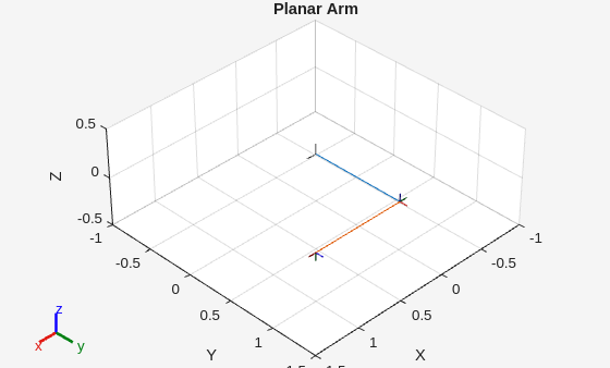
It is possible to start from a simple example, the robot below.

 1
 2
 3
 4
 5
 6
 7
 8
 9
10
11
12
13
14
15
16
17
18
19
20
21
22
23
24
25
26
27
28
29
30
31
32
33
34
35

clear
close all
clc

L1=1;
L2=1;

% a alpha d theta
dhparams = [L1      0      0      0; 
            L2      0      0      0];

%Definition of rigidBodyTree object
planar_arm=rigidBodyTree('DataFormat', 'row');
planar_arm.BaseName='base_link';

bodies=cell(size(dhparams,1)); joints=cell(size(dhparams,1));

%Generation can be iterated
for i=1:size(dhparams,1)
    %Every joint is revolute
    bodies{i}=rigidBody("link"+i);
    joints{i}=rigidBodyJoint("joint"+i, 'revolute');
    setFixedTransform(joints{i}, dhparams(i,:),'dh');
    bodies{i}.Joint=joints{i};
end

%Then joining bodies
for i=1:size(dhparams,1)
    if i==1
        addBody(planar_arm, bodies{i}, 'base_link');
    else
        addBody(planar_arm,bodies{i},bodies{i-1}.Name);
    end
end
planar_arm.showdetails

--------------------
Robot: (2 bodies)

 Idx    Body Name    Joint Name    Joint Type    Parent Name(Idx)   Children Name(s)
 ---    ---------    ----------    ----------    ----------------   ----------------
   1        link1        joint1      revolute        base_link(0)   link2(2)  
   2        link2        joint2      revolute            link1(1)   
--------------------

1
2
3
4
5

figure(1)
show(planar_arm,[pi/2 -pi/2]);
title("Planar Arm");
view([0.5 0.5 0.5]);
axis([-1.0 1.5 -1.0 1.5 -0.5 0.5]);

1
2

%Validation
T=getTransform(planar_arm, [pi/2 -pi/2], "link2")

T = 4x4
     1     0     0     1
     0     1     0     1
     0     0     1     0
     0     0     0     1

Transformation Matrix

1
2
3
4
5
6
7
8

tL1=L1;
tL2=L2;
syms theta_1 theta_2 L1 L2

A_1=[cos(theta_1) -sin(theta_1)  0 L1*cos(theta_1);
     sin(theta_1)  cos(theta_1)  0 L1*sin(theta_1);
     0             0             1 0; 
     0             0             0 1]

A_1 =

\[ \displaystyle \left(\begin{array}{cccc} \cos \left(\theta_1 \right) & -\sin \left(\theta_1 \right) & 0 & L_1 ,\cos \left(\theta_1 \right)\newline \sin \left(\theta_1 \right) & \cos \left(\theta_1 \right) & 0 & L_1 ,\sin \left(\theta_1 \right)\newline 0 & 0 & 1 & 0\newline 0 & 0 & 0 & 1 \end{array}\right) \]

1
2
3
4
5

A_2=[cos(theta_2) -sin(theta_2)  0 L2*cos(theta_2);
     sin(theta_2)  cos(theta_2)  0 L2*sin(theta_2);
     0             0             1 0; 
     0             0             0 1]

A_2 =

\[ \displaystyle \left(\begin{array}{cccc} \cos \left(\theta_2 \right) & -\sin \left(\theta_2 \right) & 0 & L_2 ,\cos \left(\theta_2 \right)\newline \sin \left(\theta_2 \right) & \cos \left(\theta_2 \right) & 0 & L_2 ,\sin \left(\theta_2 \right)\newline 0 & 0 & 1 & 0\newline 0 & 0 & 0 & 1 \end{array}\right) \]

1

T_base_ee=simplify(A_1*A_2)

T_base_ee =

\[ \displaystyle \left(\begin{array}{cccc} \cos \left(\theta_1 +\theta_2 \right) & -\sin \left(\theta_1 +\theta_2 \right) & 0 & L_2 ,\cos \left(\theta_1 +\theta_2 \right)+L_1 ,\cos \left(\theta_1 \right)\newline \sin \left(\theta_1 +\theta_2 \right) & \cos \left(\theta_1 +\theta_2 \right) & 0 & L_2 ,\sin \left(\theta_1 +\theta_2 \right)+L_1 ,\sin \left(\theta_1 \right)\newline 0 & 0 & 1 & 0\newline 0 & 0 & 0 & 1 \end{array}\right) \]

1
2
3
4
5

clear theta_1 theta_2 L1 L2
L1=tL1;
L2=tL2;
clear tL1 tL2

Solutions to the IK problem (Analytical)

Here the solution is pretty simple.

The reacheable workspace is donut-shaped. The external border is \(L_1 +L_2\), while the internal border is \(|L_1 -L_2 |\).

Given a point inside the workspace, in general, it is possible to reach the point in two configuration.

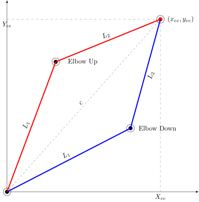
This two possibilities of configuration are called Elbow Up/Down, depending on how the solution is calculated.

Configuration 1

This configuration is called “Elbow Down” because the mid-joint is below the immaginary line joining the origin with the end-effector.

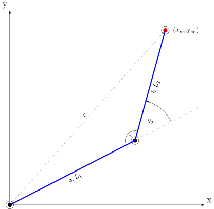
At first is needed to find \(\theta_2\), function of variables \((x_{ee} ,y_{ee} )\).

Using a generalised version of the Pythagoras’ theorem, the “Law of Cosines”:

\[ c^2 =a^2 +b^2 -2ab\cos (\gamma ) \]

And the Pythagoras formula for the right-angled triangle formed by the end-effector projection on x,y axis and the hypotenuse segment joining the origin with the end-effector:

\[ c=\sqrt{x_{ee}^2 +y_{ee}^2 } \]

It is possible to derive \(\theta_2\):

\[ \begin{array}{l} x_{ee}^2 +y_{ee}^2 ={L_1 }^2 +{L_2 }^2 -2L_1 L_2 \cos (\gamma )\newline x_{ee}^2 +y_{ee}^2 -{L_1 }^2 -{L_2 }^2 =-2L_1 L_2 \cos (\gamma )\newline \frac{x_{ee}^2 +y_{ee}^2 -{L_1 }^2 -{L_2 }^2 }{2L_1 L_2 }=-\cos (\gamma )\newline \textrm{since};\newline \theta_2 +\gamma =\pi \Rightarrow -\cos (\pi -\theta_2 )=\frac{x_{ee}^2 +y_{ee}^2 -{L_1 }^2 -{L_2 }^2 }{2L_1 L_2 }\newline \end{array} \]

\[ \begin{array}{l} \textrm{since};\newline \cos (x)=\cos (-x);\textrm{and}\cos (x+\pi )=-\cos (x)\newline \cos (\theta_2 )=\frac{x_{ee}^2 +y_{ee}^2 -{L_1 }^2 -{L_2 }^2 }{2L_1 L_2 } \end{array} \]

Arriving to the solution for \(\theta_2\)

\[ \theta_2 =\arccos \left.\Big(\frac{x_{ee}^2 +y_{ee}^2 -{L_1 }^2 -{L_2 }^2 }{2L_1 L_2 }\right.\Big) \]

Now it is possible to proceed with the calculation of \(\theta_1\).

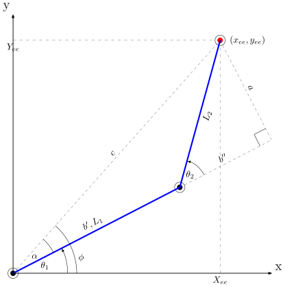
At first

\[ \theta_1 =\phi -\alpha \]

Using just a little of trigonometry

\[ \begin{array}{l} a=L_2 \sin (\theta_2 )\newline a=c\sin (\alpha )\newline b=c\cos (\alpha )\newline b^{\prime \prime } =L_2 \cos (\theta_2 )\newline \newline x_{ee} =c\cos (\phi )\newline y_{ee} =c\sin (\phi ) \end{array} \]

Expandings the equations to find \(\alpha\)

\[ \begin{array}{l} \frac{a}{b}=\frac{c\sin (\alpha )}{c\cos (\alpha )}\newline \tan (\alpha )=\frac{L_2 \sin (\theta_2 )}{b^{\prime } +b^{\prime \prime } }\newline \alpha =\arctan \Big(\frac{L_2 \sin (\theta_2 )}{L_1 +L_2 \cos (\theta_2 )}\Big) \end{array} \]

Expandings the equations to find \(\phi\)

\[ \begin{array}{l} x_{ee} =c\cos (\phi )\newline y_{ee} =c\sin (\phi )\newline \tan (\phi )=\frac{y_{ee} }{x_{ee} },~~\phi =\arctan \Big(\frac{y_{ee} }{x_{ee} }\Big) \end{array} \]

The \(\arctan\) function has some limitations, it covers only the first and the fourth quadrant.

It exists a function widely used in computer graphics and games, simulations, called atan2 that can be used to solve this problem. It covers all quadrants \((-\pi ,\pi ]\).

The atan2 function is a two-argument arctangent that returns the angle between the positive x axis and a point in the plane. Here a brief comparison between the two functions.

As reported on books and IT specifications, it is suggested to use the atan2 function instead of the traditional \(\arctan\) also because it corrects the limitations of the traditional function, correcting eventual division by zero error and adding angle correction giving the possibility to use the function on all quadrants.

Using the more robust atan2 function, the equation becomes:

\[ \phi =\textrm{atan2}(y_{ee} ,x_{ee} ) \]

\[ \alpha =\textrm{atan2}\Big(\frac{L_2 \sin (\theta_2 )}{L_1 +L_2 \cos (\theta_2 )}\Big) \]

Putting everithing togheter

\[ \theta_1 =\textrm{atan2}\Big(\frac{y_{ee} }{x_{ee} }\Big)-\textrm{atan2}\Big(\frac{L_2 \sin (\theta_2 )}{L_1 +L_2 \cos (\theta_2 )}\Big) \]

Configuration 2

Regarding the configuration Elbow Up, it is specular with respect the previous configuration. It is important to note that the angle in this configuration is negative with respect to the zero position.

\[ \cos (\theta_2 )=-\frac{x_{ee}^2 +y_{ee}^2 -{L_1 }^2 -{L_2 }^2 }{2L_1 L_2 } \]

In this configuration \(\theta_1 =\phi +\alpha\)

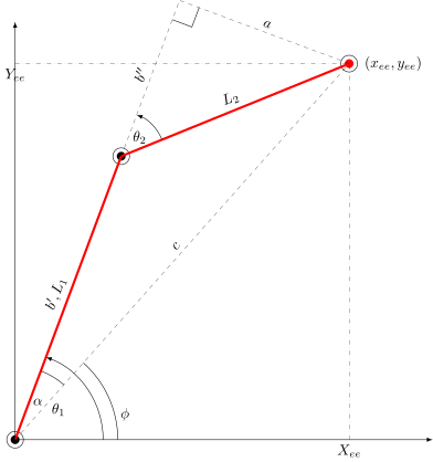
Regarding \(\phi\) and \(\alpha\), the math behind is the same of the previous case. It is verificable watching the image.

\[ \begin{array}{l} \theta_2 =-\arccos \left.\Big(\frac{x_{ee}^2 +y_{ee}^2 -{L_1 }^2 -{L_2 }^2 }{2L_1 L_2 }\right.\Big)\newline \theta_1 =\textrm{atan2}\Big(\frac{y_{ee} }{x_{ee} }\Big)+\textrm{atan2}\Big(\frac{L_2 \sin (\theta_2 )}{L_1 +L_2 \cos (\theta_2 )}\Big) \end{array} \]

Code and Validation

 1
 2
 3
 4
 5
 6
 7
 8
 9
10
11
12
13
14
15

success=true;
for i=1:10
    q=-pi+2*pi*rand(1,2);
    T=getTransform(planar_arm, q, "link2");
    qIK=twoLinkPlanarIK(1,1,T,true);
    TIK=getTransform(planar_arm, qIK, 'link2');
    if TIK ~= T
        success=false;
        disp("NOK");
    end
end

if success
    disp("Success, the function works!");
end

Success, the function works!

 1
 2
 3
 4
 5
 6
 7
 8
 9
10
11

function q = twoLinkPlanarIK(L1,L2,T,isElbowDown)
    xee=T(1,4);
    yee=T(2,4);
    sign=-1;
    if isElbowDown
        sign=1;
    end
    q2=-sign*acos((yee^2+xee^2-L1^2-L2^2)/(2*L1*L2));
    q1=atan2(yee,xee)-sign*atan2( (L2*sin(q2)) , (L1+L2*cos(q2)) );
    q=[q1,q2];
end

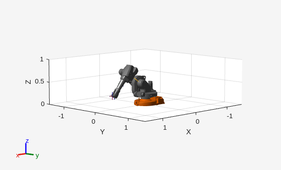
Using MATLAB IK function for 6-dof spherical wrist manipulators

ABB IRB1600

It is possible in MATLAB to import popular and well-supported robots.

1
2

abb = loadrobot("abbIrb1600",DataFormat="row");
abb.showdetails

--------------------
Robot: (7 bodies)

 Idx     Body Name           Joint Name           Joint Type     Parent Name(Idx)   Children Name(s)
 ---     ---------           ----------           ----------     ----------------   ----------------
   1        link_1              joint_1             revolute         base_link(0)   link_2(2)  
   2        link_2              joint_2             revolute            link_1(1)   link_3(3)  
   3        link_3              joint_3             revolute            link_2(2)   link_4(4)  
   4        link_4              joint_4             revolute            link_3(3)   link_5(5)  
   5        link_5              joint_5             revolute            link_4(4)   link_6(6)  
   6        link_6              joint_6             revolute            link_5(5)   tool0(7)  
   7         tool0        joint_6-tool0                fixed            link_6(6)   
--------------------

1

aIK=analyticalInverseKinematics(abb)

aIK = 
  analyticalInverseKinematics with properties:

             KinematicGroup: [1x1 struct]
              RigidBodyTree: [1x1 rigidBodyTree]
         KinematicGroupType: 'RRRSSS'
    KinematicGroupConfigIdx: [1 2 3 4 5 6]
          IsValidGroupForIK: 1

1

aIK.showdetails

--------------------
Robot: (7 bodies)

Index      Base Name   EE Body Name     Type                    Actions
-----      ---------   ------------     ----                    -------
    1      base_link         link_6   RRRSSS   Use this kinematic group
    2      base_link          tool0   RRRSSS   Use this kinematic group

If the robot is a serial chain, has 6 degrees of freedom and has a spherical wrist, it is possible to use a MATLAB function that simplify the process of controlling the robot using analyticalInverseKinematics. Otherwise it is possible to use the function generalizedInverseKinematics, but it is generally slower.

1

disp("Joint type: "+abb.getBody("tool0").Joint.Type)

Joint type: fixed

1
2
3
4
5
6
7

%Selectiong the standard TCP, fixed to the last link

%Transfer function base to TCP
%T=abb.getBody("tool0").Joint.JointToParentTransform;

%Inverse Kinematics
aIK=analyticalInverseKinematics(abb)

aIK = 
  analyticalInverseKinematics with properties:

             KinematicGroup: [1x1 struct]
              RigidBodyTree: [1x1 rigidBodyTree]
         KinematicGroupType: 'RRRSSS'
    KinematicGroupConfigIdx: [1 2 3 4 5 6]
          IsValidGroupForIK: 1

1

aIK.showdetails

--------------------
Robot: (7 bodies)

Index      Base Name   EE Body Name     Type                    Actions
-----      ---------   ------------     ----                    -------
    1      base_link         link_6   RRRSSS   Use this kinematic group
    2      base_link          tool0   RRRSSS   Use this kinematic group

1

abbIKFn = aIK.generateIKFunction("ikIRB1600")

abbIKFn = function_handle with value:
    @ikIRB1600

1
2
3

%Calculation
%Desired T
target=trvec2tform([1 0 0.3])*eul2tform([0 pi/2 0])

target = 4x4
    0.0000         0    1.0000    1.0000
         0    1.0000         0         0
   -1.0000         0    0.0000    0.3000
         0         0         0    1.0000

1
2

%Joint Positions:
qsol=abbIKFn(target)

qsol = 2x6
   -0.0000    0.9729   -0.1150    3.1416    0.8579    3.1416
   -0.0000    0.9729   -0.1150   -0.0000   -0.8579    0.0000

1
2
3
4
5
6

%Verifying
for i=1:size(qsol,1)
    disp("T from vector")
    qsol(i,:)
    disp(abb.getTransform(qsol(i,:),"tool0"))
end

T from vector
ans = 1x6
   -0.0000    0.9729   -0.1150    3.1416    0.8579    3.1416

    0.0000   -0.0000    1.0000    1.0000
    0.0000    1.0000    0.0000   -0.0000
   -1.0000    0.0000    0.0000    0.3000
         0         0         0    1.0000
T from vector
ans = 1x6
   -0.0000    0.9729   -0.1150   -0.0000   -0.8579    0.0000

    0.0000   -0.0000    1.0000    1.0000
    0.0000    1.0000    0.0000   -0.0000
   -1.0000    0.0000    0.0000    0.3000
         0         0         0    1.0000

1
2

show(abb,qsol(1,:));
axis([-1.5,1.5,-1.5,1.5,0,1])

Using MATLAB for general IK solutions

If the manipulator has more (or less or equal) than 6 joints, does not have spherical wrist, and has a more or less complex structure, it is possible to use the inverseKinematics function.

3-Link Arm

 1
 2
 3
 4
 5
 6
 7
 8
 9
10
11
12
13
14
15
16
17
18
19
20
21
22
23
24
25
26
27
28
29
30
31
32
33

L1=0.35;   
L2=0.6;   
L3=0.6;   

% a alpha d theta
dhparams = [0       pi/2   L1     0;
            L2      0      0      0; 
            L3      0      0      0];

%Definition of rigidBodyTree object
threeLinkArm=rigidBodyTree('DataFormat', 'row');
threeLinkArm.BaseName='base_link';

clear bodies joints;
bodies=cell(size(dhparams,1)); joints=cell(size(dhparams,1));

%Generation can be iterated
for i=1:size(dhparams,1)
    %Every joint is revolute
    bodies{i}=rigidBody("link"+i);
    joints{i}=rigidBodyJoint("joint"+i, 'revolute');
    setFixedTransform(joints{i}, dhparams(i,:),'dh');
    bodies{i}.Joint=joints{i};
end

%Then joining bodies
for i=1:size(dhparams,1)
    if i==1
        addBody(threeLinkArm, bodies{i}, 'base_link');
    else
        addBody(threeLinkArm,bodies{i},bodies{i-1}.Name);
    end
end

The inverseKinematics function, creates a solver to calculate joint configurations for a desired end-effector pose. It is possible to use three different algorithms.

Due to the reduced number of degrees of freedom, it is obvious that it is not possible to impose a desired attitude to the end effector but it is possible to impose a position inside the workspace.

It is also obvious to put \({\text{initialGuess}}_{\text{k}} ={\text{initialGuess}}_{\text{k-1}}\) for smoothness and simplicity in solving when using this function inside a trajectory planning cycle.

1
2
3

threeIK=inverseKinematics('RigidBodyTree',threeLinkArm);
initialGuess=[0 0 0];
T_target=trvec2tform([0.4 0.3 1])*eul2tform([0 pi/2 0])

T_target = 4x4
    0.0000         0    1.0000    0.4000
         0    1.0000         0    0.3000
   -1.0000         0    0.0000    1.0000
         0         0         0    1.0000

1
2
3
4
5

%Importance to give to rpy, xyz
weights=[0 0 0 100 100 100];

%[configSol,solInfo] = ik(endeffector,pose,weights,initialguess)
[qsol,solInfo]=threeIK("link3",T_target,weights,initialGuess)

qsol = 1x3
    0.6435    0.0967    1.6368

solInfo = struct with fields:
           Iterations: 18
    NumRandomRestarts: 0
        PoseErrorNorm: 5.8508e-07
             ExitFlag: 1
               Status: 'success'

1

T_obtained=getTransform(threeLinkArm, qsol(1,:), "link3")

T_obtained = 4x4
   -0.1296   -0.7894    0.6000    0.4000
   -0.0972   -0.5921   -0.8000    0.3000
    0.9868   -0.1620    0.0000    1.0000
         0         0         0    1.0000

Path

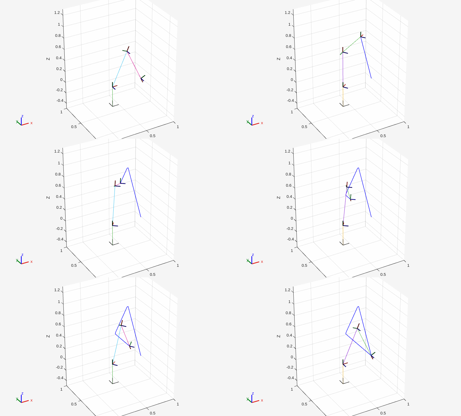
Just as a demonstration in this paragraph will be showed how to perform a simple drawing of a triangle in the \(yz\) plane at \(x=0.5\) coordinate.

Path design

 1
 2
 3
 4
 5
 6
 7
 8
 9
10
11
12
13
14
15
16
17
18
19
20
21
22
23
24
25
26
27
28
29
30
31
32
33
34
35
36
37
38
39
40
41
42
43
44
45
46
47
48
49
50
51

homePoint=[1.2,0,0.35];

triangleStartingPoint=homePoint(3);
triangleLenght=0.8;

m=tan(deg2rad(60));
q=triangleStartingPoint;

side=0:0.001:triangleLenght;

middle=round(size(side,2)/2);

total_pts=size(side,2);
Px=zeros(1,size(side,2));
Py=zeros(1,size(side,2));
Pz=zeros(1,size(side,2));

%From A to B
for i=1:middle
    Px(i)=0.5;
    Py(i)=side(i);
    Pz(i)=m*side(i)+q; 
end

A.x=Px(1);
A.y=Py(1);      
A.z=Pz(1);

B.x=Px(middle); 
B.y=Py(middle); 
B.z=Pz(middle);
%From B to C
for i=(middle+1):size(side,2)
    Px(i)=0.5;
    Py(i)=side(i);
    Pz(i)=-m*(side(i)-triangleLenght)+q;
end

C.x=Px(end);
C.y=Py(end);
C.z=Pz(end);

%From C to A
Px=[Px 0.5*ones(1,size(side,2))];
Py=[Py flip(side)];
Pz=[Pz q*ones(1,size(side,2))];

T_traj=cell(1,size(Pz,2));
for i=1:size(T_traj,2)
    T_traj{i}=trvec2tform([Px(i) Py(i) Pz(i)])*eul2tform([0 0 0]);
end

Inverse Kinematics for obtaining angles

 1
 2
 3
 4
 5
 6
 7
 8
 9
10
11
12
13
14
15
16
17
18
19
20
21

threeIK=inverseKinematics('RigidBodyTree',threeLinkArm);

%The starting point is near the homePoint, it is possible to leave this
%value unaltered
initialGuess=[0 0 0];

%Importance to give to rpy, xyz
weights=[0 0 0 100 100 100];
q_triangle=cell(1,size(T_traj,2));

for i=1:size(T_traj,2)
    %[configSol,solInfo] = ik(endeffector,pose,weights,initialguess)
    [qsol,solInfo]=threeIK("link3",T_traj{i},weights,initialGuess);
    
    q_triangle{i}=qsol(1,:);
    if solInfo.Status~='success'
        disp("Error during IK");
    end
    %Current position is the best initialGuess for the next iteration
    initialGuess=qsol(1,:);
end

Plotting

 1
 2
 3
 4
 5
 6
 7
 8
 9
10
11
12
13
14
15
16
17
18
19
20
21
22
23
24
25
26
27
28
29
30
31
32
33
34
35
36
37
38
39
40
41
42
43
44
45
46
47
48

% Settings %
robot=threeLinkArm;
ee_name='link3';
%row cell
q_vect=q_triangle; 
% END SETTINGS %
robot.DataFormat = 'row';
num_steps=length(q_triangle);
ee_positions=cell(1,num_steps);

for i = 1:num_steps
    tform=getTransform(threeLinkArm, q_vect{i}, ee_name);
    ee_positions{i}=tform(1:3, 4)';
end

fig=figure;
ax=axes('Parent', fig);

config_init = q_vect{1};
show(robot, config_init, 'Parent', ax, 'PreservePlot', false);

hold(ax, 'on'); 

axis(ax, 'equal');
xlim(ax, [-0.3 1]);
ylim(ax, [-0.2 1]);
zlim(ax, [-0.5 1.3]);
view(-30, 30);
grid(ax, 'on');

trace=plot3(ax, NaN, NaN, NaN, 'b-', 'LineWidth', 1);
speedUpFactor=100; 

x_trace=[];
y_trace=[];
z_trace=[];

for i=1:speedUpFactor:num_steps
    show(robot, q_vect{i}, 'Parent', ax, 'PreservePlot', false);
    ee_position=ee_positions{i};

    x_trace=[x_trace ee_position(1)];
    y_trace=[y_trace ee_position(2)];
    z_trace=[z_trace ee_position(3)];
    set(trace, 'XData', x_trace, 'YData', y_trace, 'ZData', z_trace);
    drawnow;
end
hold(ax, 'off');