Robot Definition and Direct Kinematic

It’s possible to define a robot in different ways. Every representation has its advantages in terms of simplicity, environment compatibility, modelling convenience.

A mathematical model is the simplest possible representation of the robot. It represents the robot’s kinematics and dynamics through equations to predict physical behavior. It calculates how joint movements and actuator forces translate into spatial positioning, giving a starting point for developing simulations, deciding how to control the robot’s movements and studying stability and dinamics.

It is possible to represent a robot using proprietary softwares such as SolidWorks, Fusion360, Matworks’s Simscape Multibody trought a model. We can refer to this representations with the names Digital Twins, Simulation Model, Virtual Model.

It is also possible to have a textual representation of the robot. ROS uses URDF (Unified Robot Description Format), an XML-like format. Another popular environment, WeBots, uses PROTO as language to define robots. It exists tools able to convert CAD Models to textual representation, presenving and integrating 3D meshes.

Formulas

\[ A_i^{i-1} =\left\lbrack \begin{array}{cccc} \cos \theta_i & -\sin \theta_i \cos \alpha_i & \sin \theta_i \sin \alpha_i & a_i \cos \theta_i \newline \sin \theta_i & \cos \theta_i \cos \alpha_i & -\cos \theta_i \sin \alpha_i & a_i \sin \theta_i \newline 0 & \sin \alpha_i & \cos \alpha_i & d_i \newline 0 & 0 & 0 & 1 \end{array}\right\rbrack \]

One Link Robot Definition using Peter Corke’s toolbox (RTB)

One Link Robot Math

DH-parametets

Link	\(a_i\)	\(alpha_i\)	\(theta_i\)	\(d_i\)
Link 1	1	0	\(\displaystyle \theta_1\)	0

Transfer matrix

\[ A_1^0 =\left\lbrack \begin{array}{cccc} \cos \theta_1 & -\sin \theta_1 & 0 & \cos \theta_1 \newline \sin \theta_1 & \cos \theta_1 & 0 & \sin \theta_1 \newline 0 & 0 & 1 & 0\newline 0 & 0 & 0 & 1 \end{array}\right\rbrack \]

It’s easy to demonstrate

 1
 2
 3
 4
 5
 6
 7
 8
 9
10
11
12
13


clear
close all
clc

addpath(genpath('RVC3-MATLAB'))
a1=1;
%Create a rotation around the Z-axis about an angle q1
onelink=ETS3.Rz("q1");
%Creates a homogeneous transformation 
%representing a translation along the X-axis for a length a1
onelink=onelink*ETS3.Tx(a1);
%Calculating forward kinematics
onelink.fkine(pi/2)


ans = 4x4
    0.0000   -1.0000         0    0.0000
1.0000    0.0000         0    1.0000
         0         0    1.0000         0
         0         0         0    1.0000

It is possible to show the robot structure using the method teach

1

%onelink.teach

Python version

It exsist a Python version called roboticstoolbox. Below a code example that do the same but in Python.

It’s important to use a virtual environments and install specific versions of dependant libraries (numpy==1.26.4 matplotlib==3.5.0)

 1
 2
 3
 4
 5
 6
 7
 8
 9
10
11
12
13
14
15
16
17
18
19
20
21


import numpy as np
import roboticstoolbox as rtb

#Defining parameter
a1=1
#Defining rotation around z axis, then translation towards x axis of a1
onelink=rtb.ET.Rz()*rtb.ET.tx(a1)

print("Robot structure")
print(onelink)

q=[np.pi/2]
fk_result=onelink.fkine(q)

print("\nForward kinematics (SE3):")
print(fk_result)

#Converting to Robot object for using 
#the teach(q) method
onelinkrobot=rtb.Robot(onelink, name="OneLinkRobot")
onelinkrobot.teach(q)

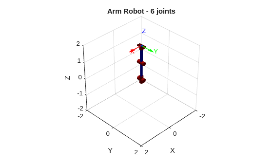
Six Link Robot using Peter Corke’s toolbox - Arm

Below a 6-DoF robot designed to mimic the human arm structure (shoulder, elbow, and wrist joints).

1
2
3
4
5


a1=1; 
a2=1;
armrobot=ETS3.Rz("q1")*ETS3.Ry("q2")*ETS3.Tz(a1)*...
    ETS3.Ry("q3")*ETS3.Tz(a2)*ETS3.Rz("q4")*ETS3.Ry("q5")*ETS3.Rz("q6");
armrobot.njoints %returns number of joints


ans = 6

1

armrobot.structure %returns structure of robot (P-Prismatic, R-Revolute, S-Spherical)


ans = 'RRRRRR'

1

armrobot.fkine(zeros(1,6))


ans = 4x4
     1     0     0     0
     0     1     0     0
     0     0     1     2
     0     0     0     1

1
2
3


figure(1)
armrobot.plot(zeros(1,6));
title("Arm Robot - 6 joints")

1

%armrobot.teach;

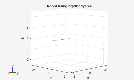
Robot definition using Rigid Body Tree

MATLAB implements some native tools too. The class rigidBodyTree gives the possibility to build robot models by connecting rigidBody objects through rigidBodyJoints. It is a versatile tool for defining a robot’s architecture and it may be preferred because it’s better integrated with the MatWorks ecosystem.

 1
 2
 3
 4
 5
 6
 7
 8
 9
10
11
12
13
14
15
16
17
18
19
20
21
22
23
24
25
26
27
28


% Documentation following
% https://mathworks.com/help/robotics/ref/rigidbodytree.html

%Defining a robot object as rigidBodyTree
%DataFormat-row defines q as a row input 
robot=rigidBodyTree('DataFormat', 'row');
robot.BaseName='base_link';
a1=1; 
a2=1;

%Defining links, joints
link1=rigidBody("link1");
link1.Joint=rigidBodyJoint("joint1","revolute");

link2=rigidBody("link2");
link2.Joint=rigidBodyJoint("joint2","revolute");
setFixedTransform(link2.Joint, se3([a1 0 0],"trvec")); %Adding link length

link3=rigidBody("link3");
link3.Joint=rigidBodyJoint("joint3","fixed"); %latest link
setFixedTransform(link3.Joint, se3([a2 0 0],"trvec"));

%Adding bodies to rigidBodyTree object
robot.addBody(link1,robot.BaseName);
robot.addBody(link2,link1.Name);
robot.addBody(link3,link2.Name);

robot.showdetails %Show table describing the Tree


--------------------
Robot: (3 bodies)

 Idx    Body Name    Joint Name    Joint Type    Parent Name(Idx)   Children Name(s)
 ---    ---------    ----------    ----------    ----------------   ----------------
   1        link1        joint1      revolute        base_link(0)   link2(2)  
   2        link2        joint2      revolute            link1(1)   link3(3)  
   3        link3        joint3         fixed            link2(2)   
--------------------

1
2
3
4



figure(2)
show(robot);
title("Robot using rigidBodyTree");

1
2
3
4



%Get relative transfer function from link2 respect link1
T=robot.getTransform([pi/6 pi/4], "link2", "link1");
T


T = 4x4
    0.7071   -0.7071         0    1.0000
    0.7071    0.7071         0         0
         0         0    1.0000         0
         0         0         0    1.0000

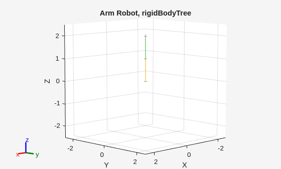
Converting Peter Corke’s Toolbox Robot to RigidBodyTree

It is possible to convert an ETS3 object (Peter Corke’s Toolbox) to a MATLAB standard rigidBodyTree object. Despite the RTB is simpler to use, it’s generically considered better to use the standard implementation.

1
2
3
4


armbotbodytree=ets2rbt(armrobot);
figure(3)
show(armbotbodytree);
title("Arm Robot, rigidBodyTree");

Using DH Parameters - MATLAB’s Toolbox

Using this aproach it-s possible to define a robot starting from the DH parameters.

The main code requires the definition of the rigidBodyTree object, then creating bodies and connecting to the base in the end.

Here an example.

Link	\(alpha_i\)	\(theta_i\)	\(d_i\)
1	0	0	\(\displaystyle q_1\)
2	\(\displaystyle -\frac{\pi }{2}\)	\(\displaystyle q_2\)	0
3	0	\(\displaystyle q_3\)	0

 1
 2
 3
 4
 5
 6
 7
 8
 9
10
11
12
13
14
15
16
17
18
19
20
21
22
23
24
25
26
27
28
29
30
31
32
33
34
35
36
37
38
39
40
41


% Documentation following
% https://it.mathworks.com/help/robotics/ug/build-manipulator-robot-using-kinematic-dh-parameters.html
%Definition of the DH parameter matrix 
clear
clc

% a alpha d theta
dhparams = [0      0      0      0; 
            0      -pi/2  0      0; 
            0      0      0      0];
%Definition of rigidBodyTree object
cyl_arm=rigidBodyTree('DataFormat', 'row');
cyl_arm.BaseName='base_link';

bodies=cell(size(dhparams,1)); joints=cell(size(dhparams,1));

%Generation can be iterated
for i=1:size(dhparams,1)
    %Only for the first joint that is revolute
    if i==1
        bodies{i}=rigidBody("link"+i);
        joints{i}=rigidBodyJoint("joint"+i, 'revolute');
        setFixedTransform(joints{i}, dhparams(i,:),'dh');
        bodies{i}.Joint=joints{i};
    else
        bodies{i}=rigidBody("link"+i);
        joints{i}=rigidBodyJoint("joint"+i, 'prismatic');
        setFixedTransform(joints{i}, dhparams(i,:),'dh');
        bodies{i}.Joint=joints{i};
    end
end

%Then joining bodies
for i=1:size(dhparams,1)
    if i==1
        addBody(cyl_arm, bodies{i}, 'base_link');
    else
        addBody(cyl_arm,bodies{i},bodies{i-1}.Name);
    end
end
cyl_arm.showdetails


--------------------
Robot: (3 bodies)

 Idx    Body Name    Joint Name    Joint Type    Parent Name(Idx)   Children Name(s)
 ---    ---------    ----------    ----------    ----------------   ----------------
   1        link1        joint1      revolute        base_link(0)   link2(2)  
   2        link2        joint2     prismatic            link1(1)   link3(3)  
   3        link3        joint3     prismatic            link2(2)   
--------------------

1
2
3


figure(4)
show(cyl_arm,[pi/2 1 1.5]);
title("Cylindical Arm");

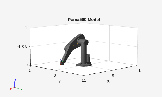
Puma 560 Robot

The PUMA (Programmable Universal Machine for Assembly) is one of the most iconic and influential industrial robots in history. Originally designed for General Motors to assemble small automobile components, now it’s commonly used as a didactic example.

DH Puma 560	\(\displaystyle a\)	\(\displaystyle \alpha\)	\(\displaystyle d\)	\(\displaystyle \theta\)
1	0	\(\displaystyle \frac{\pi }{2}\)	0	q1
2	0.4318	0	0	q2
3	0.0203	\(\displaystyle -\frac{\pi }{2}\)	0.15005	q3
4	0	\(\displaystyle \frac{\pi }{2}\)	0.4318	q4
5	0	\(\displaystyle -\frac{\pi }{2}\)	0	q5
6	0	0	0	q6

 1
 2
 3
 4
 5
 6
 7
 8
 9
10
11
12
13
14
15
16
17
18
19
20
21
22
23
24
25
26
27
28
29
30
31
32
33
34
35
36
37
38
39
40
41
42


clear
clc

% Documentation following
% https://it.mathworks.com/help/robotics/ug/build-manipulator-robot-using-kinematic-dh-parameters.html

%Definition of the DH parameter matrix 
dhparams = [0         pi/2         0         0; 
            0.4318    0            0         0; 
            0.0203   -pi/2         0.15005   0;
            0         pi/2         0.4318    0;
            0        -pi/2         0         0;
            0         0            0         0];
%Definition of rigidBodyTree object
puma=rigidBodyTree('DataFormat', 'row');
puma.BaseName='base_link';

bodies=cell(size(dhparams,1)); joints=cell(size(dhparams,1));

%Generation can be iterated
for i=1:size(dhparams,1)
    %Every joint is revolute
    bodies{i}=rigidBody("link"+i);
    joints{i}=rigidBodyJoint("joint"+i, 'revolute');
    setFixedTransform(joints{i}, dhparams(i,:),'dh');
    bodies{i}.Joint=joints{i};
end

%Then joining bodies
for i=1:size(dhparams,1)
    if i==1
        addBody(puma, bodies{i}, 'base_link');
    else
        addBody(puma,bodies{i},bodies{i-1}.Name);
    end
end
figure(5)
show(puma);
title("Puma 560 Robot, rigidBodyTree");

%It is possible to interact with the robot using
%interactiveRigidBodyTree(puma)

Loading Existing Models

Custom or OEM robot models can be loaded in to the MATLAB workspace.

It is possible to find some opensource models about the most popular ones following this link.

Matlab’s Robotics System Toolbox has a lot of models that can be loaded using the function loadrobot, including meshes, inertia, mechanical limitations and more.

Documentation about the function can be found here.

1
2
3
4
5


clear
clc

puma560=loadrobot("puma560","DataFormat","row");
puma560.showdetails


--------------------
Robot: (6 bodies)

 Idx    Body Name   Joint Name   Joint Type    Parent Name(Idx)   Children Name(s)
 ---    ---------   ----------   ----------    ----------------   ----------------
   1        link2           j1     revolute            link1(0)   link3(2)  
   2        link3           j2     revolute            link2(1)   link4(3)  
   3        link4           j3     revolute            link3(2)   link5(4)  
   4        link5           j4     revolute            link4(3)   link6(5)  
   5        link6           j5     revolute            link5(4)   link7(6)  
   6        link7           j6     revolute            link6(5)   
--------------------

1
2
3
4
5


q=[0 -pi/8 -2*pi/3 0 2*pi/3 pi/5];
figure(6)
show(puma560,q);
axis([-1,1,-1,1,0,1])
title("Puma560 Model")

It is possible to interact with the robot using:

1

interactiveRigidBodyTree(puma560)