Unicycle Model

Introduction
Unicycle

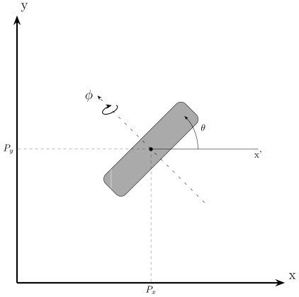
Kinematic model of an unicycle:

\[ \begin{array}{l} \left\lbrack \begin{array}{c} \dot{x} \newline \dot{y} \newline \dot{\theta} \end{array}\right\rbrack =\left\lbrack \begin{array}{cc} r\cos (\theta ) & 0\newline r\sin (\theta ) & 0\newline 0 & 1 \end{array}\right\rbrack \left\lbrack \begin{array}{c} \dot{\phi} \newline \omega \end{array}\right\rbrack \ \ \ \ \left\lbrack \begin{array}{c} \dot{x} \newline \dot{y} \newline \dot{\theta} \end{array}\right\rbrack \ \text{from the state} \ q=\left\lbrack \begin{array}{c} x\newline y\newline \theta \end{array}\right\rbrack \ \end{array} \]

It’s possible to control the vehicle using \(v\) and \(\omega\) as used in the ROS topic cmd_vel using this formulation:

\[ \left\lbrack \begin{array}{c} \dot{x} \newline \dot{y} \newline \dot{\theta} \end{array}\right\rbrack =\left\lbrack \begin{array}{cc} \cos (\theta ) & 0\newline \sin (\theta ) & 0\newline 0 & 1 \end{array}\right\rbrack \left\lbrack \begin{array}{c} v\newline \omega \end{array}\right\rbrack \]

This is the basic mobile robot model

Code

The simulation will use the ode45 solver.

 1
 2
 3
 4
 5
 6
 7
 8
 9
10
11
12
13
14
15
16
17
18
19
20
21
22
23
24
25
26
27
28
29
30
31
32
% Documentation following 
% https://mathworks.com/help/robotics/ref/unicyclekinematics.html
% The simulation will use ode45 solver
%  [t,y] = ode45(@(t,y)derivative(kinematicModel,y,inputs),tspan,initialState);
clear
close all
clc

%Unicycle model
unicycleModel=unicycleKinematics;
unicycleModel.VehicleInputs='VehicleSpeedHeadingRate'; %[v w]'

%Setting parameters
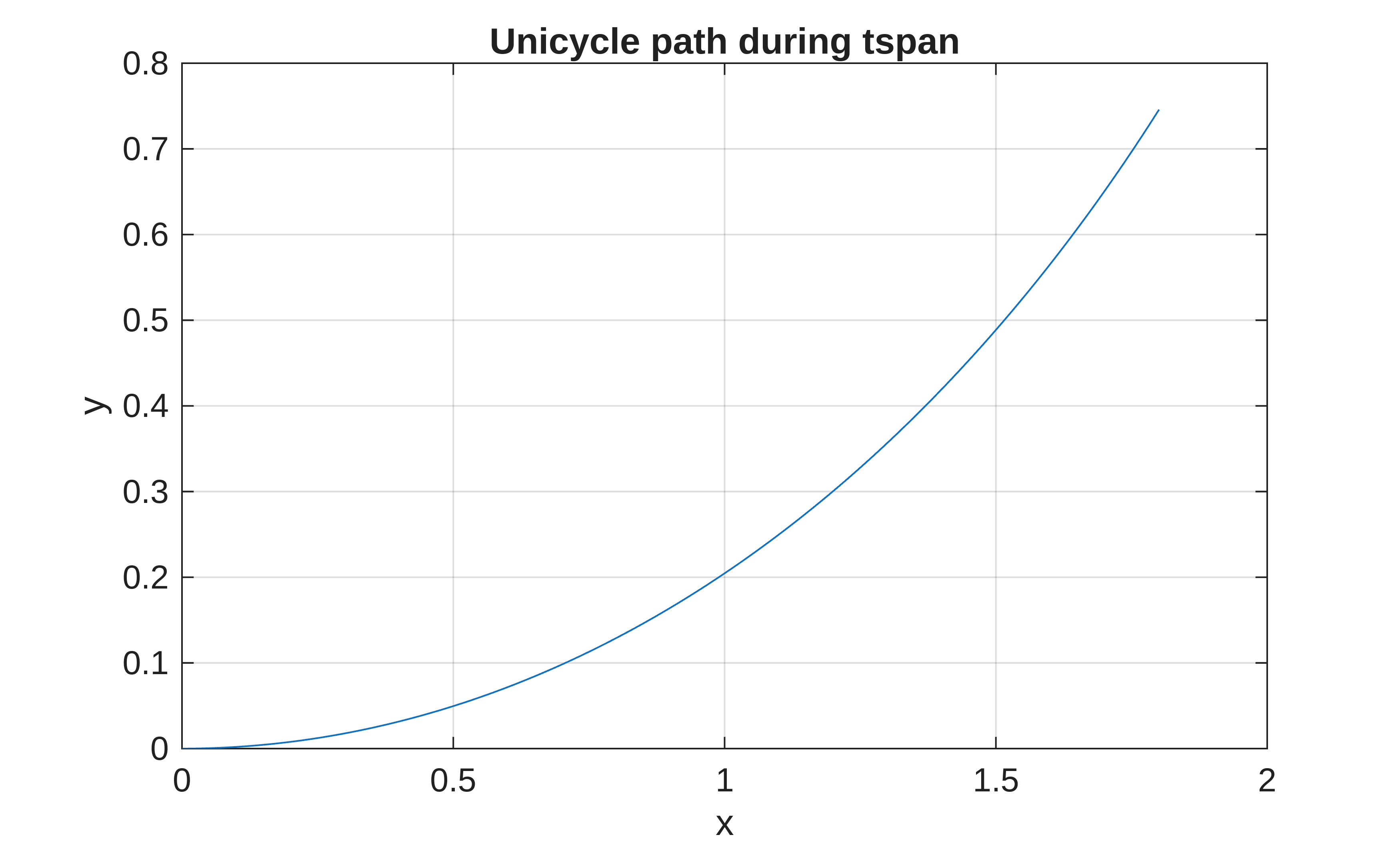
tspan=0:5e-3:1; %Simulation time 
initialState=[0 0 0]; %[x, y, theta]
inputs=[2 pi/4]; %[v w]

[t,y]=ode45(@(t,y)derivative(unicycleModel,y,inputs),tspan,initialState);
q=y;
q_u=q;

%Decomposing q into its variables
x=q(:,1);
y=q(:,2);
theta=q(:,3);

%Plotting Results
figure(1)
plot(x, y), grid on
title("Unicycle path during tspan")
xlabel("x")
ylabel("y")
Unicycle path

Bicycle Model

Introduction

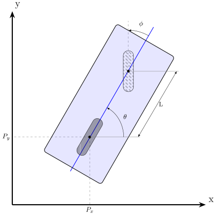
Bicycle

The bicycle model is defined by the following equation

\[ \left\lbrack \begin{array}{c} \dot{x} \newline \dot{y} \newline \dot{\theta} \newline \dot{\phi} \end{array}\right\rbrack =\left\lbrack \begin{array}{cc} \cos (\theta ) & 0\newline \sin (\theta ) & 0\newline \frac{\tan (\phi )}{L} & 0\newline 0 & 1 \end{array}\right\rbrack \left\lbrack \begin{array}{c} v\newline \omega \end{array}\right\rbrack \]

Where v is vehicle speed and omega is the stering angle

If it is possible to directly control the stering angle phi, then the model become:

\[ \begin{array}{l} \left\lbrack \begin{array}{c} \dot{x} \newline \dot{y} \newline \dot{\theta} \end{array}\right\rbrack =\left\lbrack \begin{array}{cc} \cos (\theta ) & 0\newline \sin (\theta ) & 0\newline 0 & 1 \end{array}\right\rbrack \left\lbrack \begin{array}{c} v\newline \widehat{\omega} \end{array}\right\rbrack \\ \\ \widehat{\omega} =\frac{v}{L}\tan (\phi ) \end{array} \]

The ideal center of the robot is inside the motored wheel.

It’s important to remeber to set the L parameter.

Code

 1
 2
 3
 4
 5
 6
 7
 8
 9
10
11
12
13
14
15
16
17
18
19
20
21
22
23
24
25
26
27
28
29
% Documentation following 
% https://it.mathworks.com/help/robotics/ref/bicyclekinematics.html
% The simulation will use ode45 solver
%  [t,y] = ode45(@(t,y)derivative(kinematicModel,y,inputs),tspan,initialState);

%% Bicycle model
bicycleModel=bicycleKinematics;
bicycleModel.VehicleInputs=...
    'VehicleSpeedHeadingRate'; %[v, w_hat]
bicycleModel.WheelBase=1; % Front-Rear wheel distance (default is 1)

%Setting parameters
tspan=0:5e-3:1;
initialState=[0 0 0]; %[x,y,theta]
inputs=[2 pi/4]; %[v, w_hat]
[t,y] = ode45(@(t,y)derivative(bicycleModel,y,inputs),tspan,initialState);
q=y;
q_b=q;
%Decomposing q into its variables
x=q(:,1);
y=q(:,2);
theta=q(:,3);

%Plotting Results
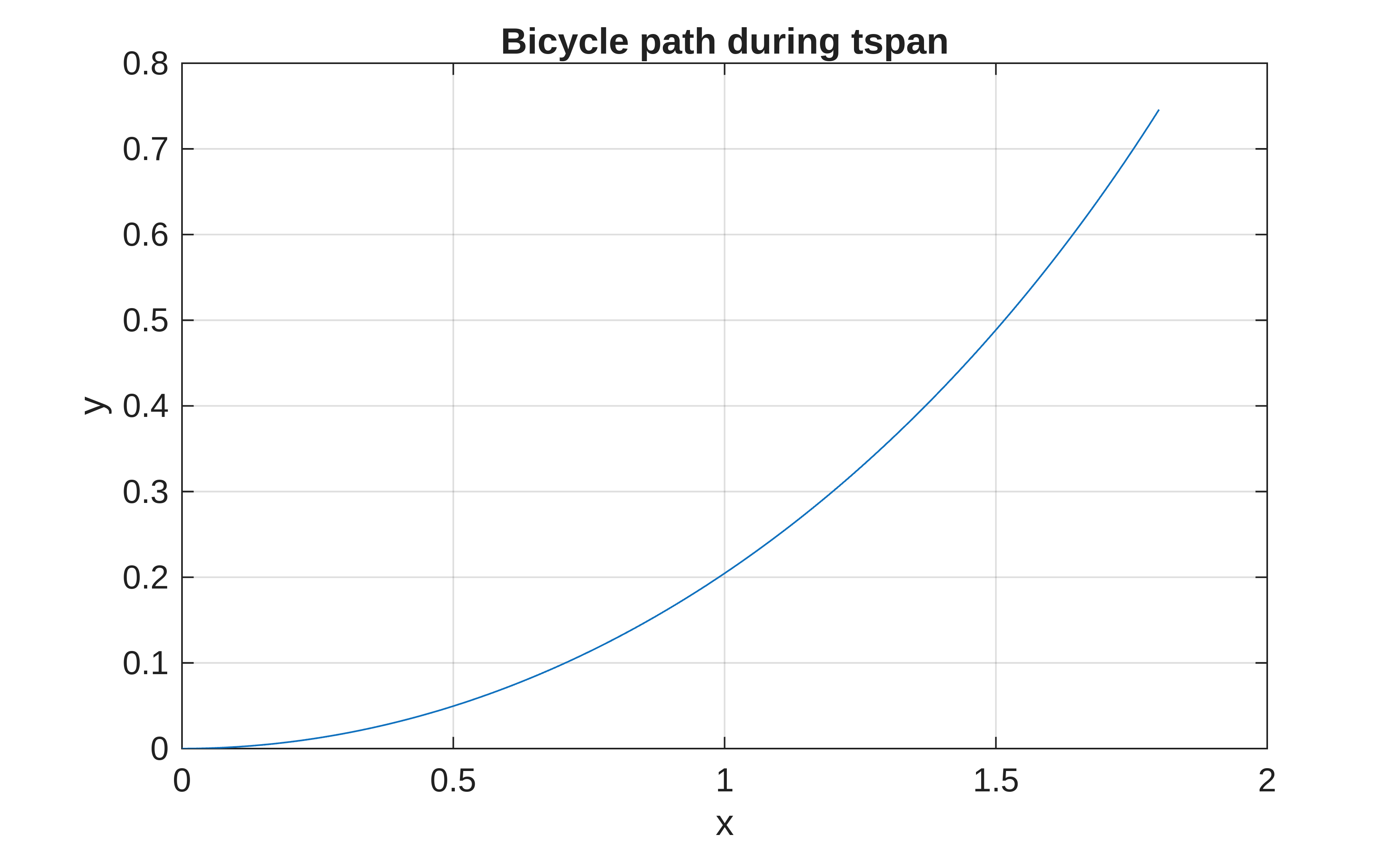
figure(2)
plot(x,y), grid on
title("Bicycle path during tspan")
xlabel("x")
ylabel("y")
Bicycle Graph

Differential Drive (Roomba style)

Introduction

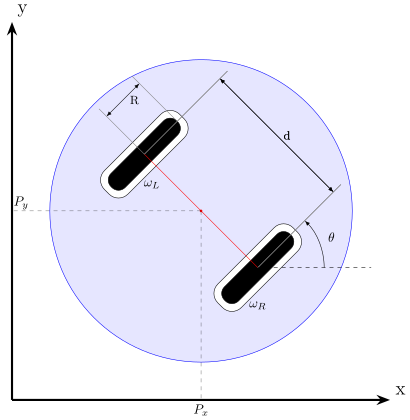
The differential drive robot model is a practical physical implementation of the kinematic unicycle model. It is based on decomposing the ideal unicycle into two independently actuated components. By separately controlling two driving wheels, the robot generates linear and rotational movements equivalent to those of a unicycle.
DiffDrive

The front velocity will be the resulting composition of the effects from both left and right wheel angular velocity \(v=\frac{R(\omega_L +\omega_R )}{2}\).

Similar considerations apply to the resulting angular velocity, though with distinct operational differences. It is essential to maintain the right hand rule convention during formulation. In addition, one must note that the resulting angular momentum decreases as the distance between the wheels increases \(\omega =\frac{R(\omega_R -\omega_L )}{d}\).

\[ \begin{array}{l} \left\lbrack \begin{array}{c} \dot{x} \newline \dot{y} \newline \dot{\theta} \end{array}\right\rbrack =\left\lbrack \begin{array}{cc} \cos (\theta ) & 0\newline \sin (\theta ) & 0\newline 0 & 1 \end{array}\right\rbrack \left\lbrack \begin{array}{c} v\newline \omega \end{array}\right\rbrack \\ \\ v=\frac{R(\omega_L +\omega_R )}{2},~\omega =\frac{R(\omega_R -\omega_L )}{d} \end{array} \]

The center of the robot is located on the middle point beetween the wheel axis. Usually some passive supports are added to maintain equilibrium (like a castor wheel or a spherical wheel).

It is possible to define wheel radius and distance. If controlled trought \(\left\lbrack \begin{array}{c} v\newline \omega \end{array}\right\rbrack\) the results will be the same of the unicycle. Those parameters will then have effects on \(\omega_R\) and \(\omega_L\).

Code

 1
 2
 3
 4
 5
 6
 7
 8
 9
10
11
12
13
14
15
16
17
18
19
20
21
22
23
24
25
26
27
28
29
30
31
32
% Documentation following 
% https://it.mathworks.com/help/robotics/ref/differentialdrivekinematics.html
% The simulation will use ode45 solver
%  [t,y] = ode45(@(t,y)derivative(kinematicModel,y,inputs),tspan,initialState);

diffdriveModel=differentialDriveKinematics;
diffdriveModel.WheelRadius=0.05; %R
diffdriveModel.TrackWidth=0.2; %d
diffdriveModel.VehicleInputs='VehicleSpeedHeadingRate'; %[v w]'
% It is possible to simulate using wheel speed only
%diffdriveModel.VehicleInputs='WheelSpeed'; %[v_r v_l]'

%Setting parameters
tspan=0:5e-3:1; %Simulation time 
initialState=[0 0 0]; %[x, y, theta]
inputs=[2 pi/4]; %[v w]

[t,y] = ode45(@(t,y)derivative(diffdriveModel,y,inputs),tspan,initialState);

q=y;
q_d=q;
%Decomposing q into its variables
x=q(:,1);
y=q(:,2);
theta=q(:,3);

%Plotting Results
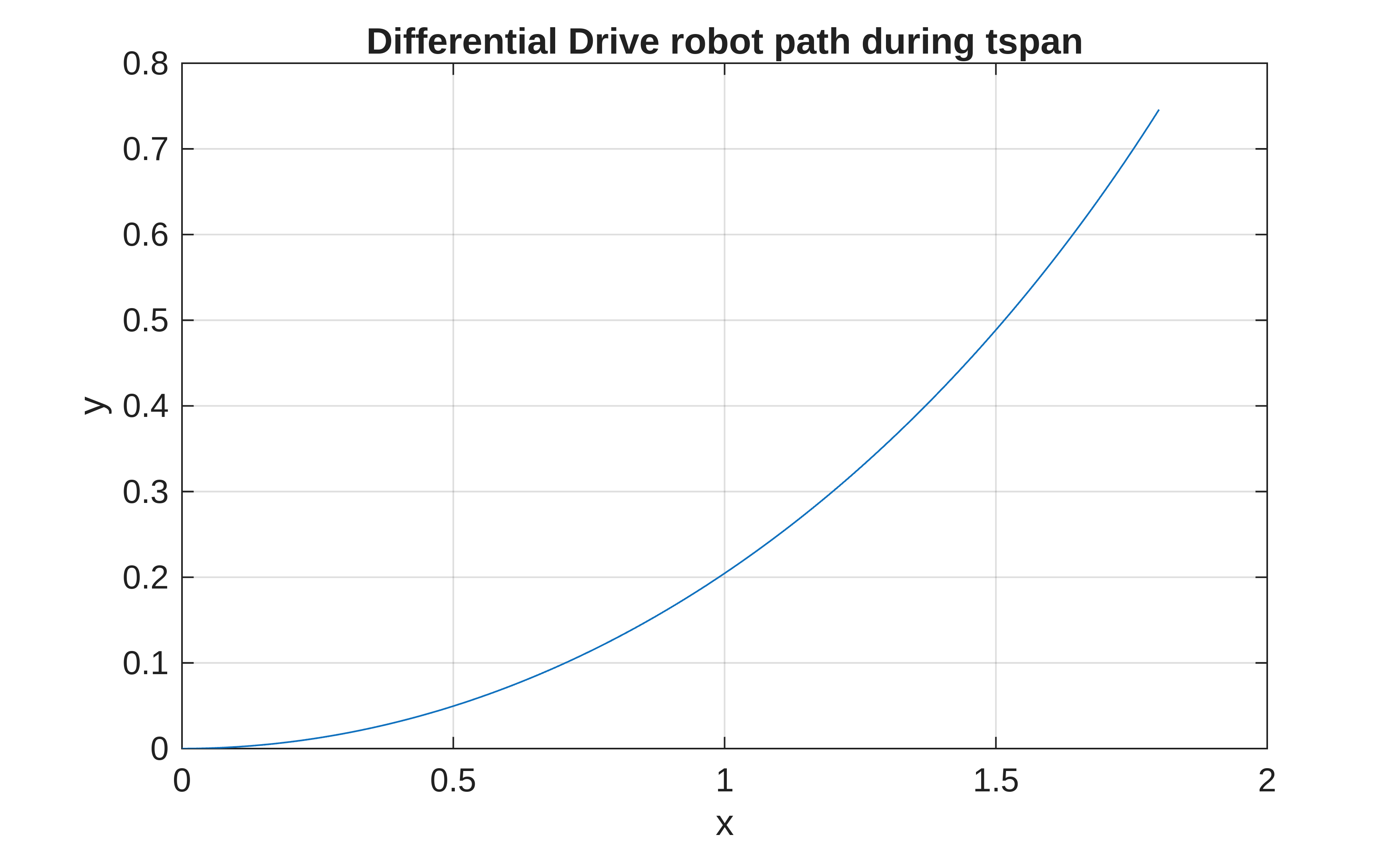
figure(3)
plot(x,y), grid on
title("Differential Drive robot path during tspan")
xlabel("x")
ylabel("y")
DiffDrive Path

Model From Scratch

It is useful know how to derive and simulate a mobile robot kinematic model from first principles, entirely without relying on specialized robotics toolboxes. Developing a barebone model manually forces a deeper understanding of the system’s physics and eliminates restrictive software dependencies.

More importantly, this approach frees the code from proprietary platforms like MATLAB, making the core equations universally portable and easily translatable to open-source environments, custom software nodes, or directly into low-level embedded hardware.

Implementation of the Unicycle Model

 1
 2
 3
 4
 5
 6
 7
 8
 9
10
11
12
13
14
15
16
17
18
function dq=UnicycleModel(t,q,mode)
    %x=q(1);
    %y=q(2);
    %theta=q(3);
    
    inputs=[2 pi/4]'; %[v w]
    %Using angular velocity
    %inputs=[2*pi pi/4]'; %[phi_dot w]

    %Radius Parameter
    r=1;

    %Using angular speed [rad/s]
    %dq=[r*cos(theta) 0; r*sin(theta) 0; 0 1]*inputs;

    %Using linear velocity [m/s]
    dq=[cos(q(3)) 0; sin(q(3)) 0; 0 1]*inputs;
end

Implementation of the Bicycle Model

 1
 2
 3
 4
 5
 6
 7
 8
 9
10
11
12
13
14
15
16
17
18
function dq=BicycleModel(t,q)
    %x=q(1);
    %y=q(2);
    %theta=q(3);
    %phi=q(4);

    inputs=[2 pi/4]'; %[v w_hat]
    %inputs=[2 pi/4]'; %[v w]

    %Radius Parameter
    r=0.34;
    l=1;
    %Using angular speed [rad/s]
    %dq=[cos(theta) 0; sin(theta) 0; tan(q(4))/L 0; 0 1]*inputs;

    %Using linear velocity [m/s]
    dq=[cos(q(3)) 0; sin(q(3)) 0; 0 1]*inputs;
end

Implementation of the Differential Drive Model

 1
 2
 3
 4
 5
 6
 7
 8
 9
10
11
12
13
14
15
16
17
18
19
20
function dq=DiffDriveModel(t,q)
    %x=q(1);
    %y=q(2);
    %theta=q(3);
    
    inputs=[2 pi/4]'; %[v w]
    %inputs=[2*pi 2*pi]'; %[r_angular_speed l_angular_speed]

    %Radius and Distance Parameters
    r=0.05;
    d=0.2;

    %Using angular speed for left and rigt [rad/s]
    %dq=[(r/2)*cos(q(3)) (r/2)*cos(q(3));
    %    (r/2)*sin(q(3)) (r/2)*sin(q(3)); 
    %    -r/d             r/d]*inputs;

    %Using linear velocity [m/s]
    dq=[cos(q(3)) 0; sin(q(3)) 0; 0 1]*inputs;
end

Validating Result

 1
 2
 3
 4
 5
 6
 7
 8
 9
10
11
12
13
14
15
16
17
18
19
20
21
22
23
24
25
26
27
28
29
30
31
32
33
34
35
% https://it.mathworks.com/help/matlab/ref/ode45.html
% [t,y] = ode45(odefun,tspan,y0)
% Where odefun is a set of differential equations
%  function dydt = odefun(t,y)
%   dydt = zeros(2,1);
%   dydt(1) = y(1)+2*y(2);
%   dydt(2) = 3*y(1)+2*y(2);
%  end
tspan=0:5e-3:1; %Simulation time 
initialState=[0 0 0]; %[x, y, theta]

%[t_tbox,q_tbox] = ode45(@(t_tbox,y_tbox) ...
%    derivative(unicycleModel,y_tbox,inputs),tspan,initialState);
[t_cust_u,q_cust_u] = ode45(@UnicycleModel,tspan,initialState);
[t_cust_b,q_cust_b] = ode45(@BicycleModel,tspan,initialState);
[t_cust_d,q_cust_d] = ode45(@DiffDriveModel,tspan,initialState);

figure(4);
subplot(2, 3, 1);
plot(q_u(:,1), q_u(:,2), 'r');
title('Unicycle');
ylabel('Toolbox', 'FontWeight', 'bold');
subplot(2, 3, 2);
plot(q_b(:,1), q_b(:,2), 'g');
title('Bicycle');
subplot(2, 3, 3);
plot(q_d(:,1), q_d(:,2), 'b');
title('DiffDrive');
subplot(2, 3, 4);
plot(q_cust_u(:,1), q_cust_u(:,2), 'm');
ylabel('Custom', 'FontWeight', 'bold');
subplot(2, 3, 5);
plot(q_cust_b(:,1), q_cust_b(:,2), 'y');
subplot(2, 3, 6);
plot(q_cust_d(:,1), q_cust_d(:,2), 'c');
CustPlot

Considerations

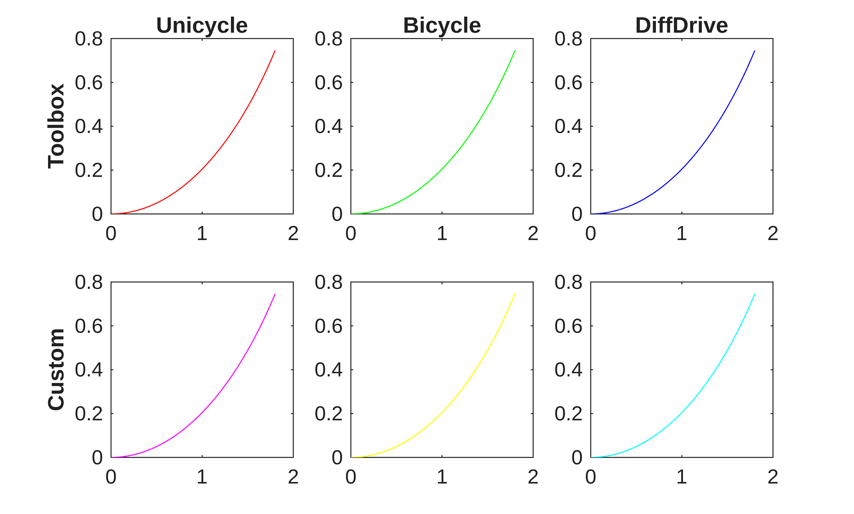
By controlling using \(\left\lbrack \begin{array}{c} v\newline \omega \end{array}\right\rbrack\) we see that unicycle and differencial drive robots have basically the same output. The parameter L on the bicycle model is considerably influencing the path.

Using Simulink

Simulink provides a GUI helping dealing with this models.

Sim GUI

Opening the corresponding block it is possible to configure it as previously done in code.
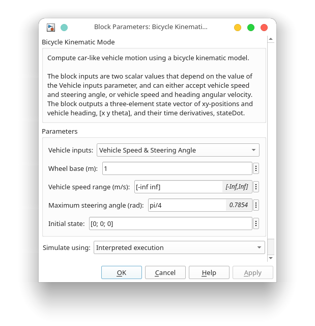
Conf

Using the Simulink interface can be preferred for its simplicity and immediacy during developement.

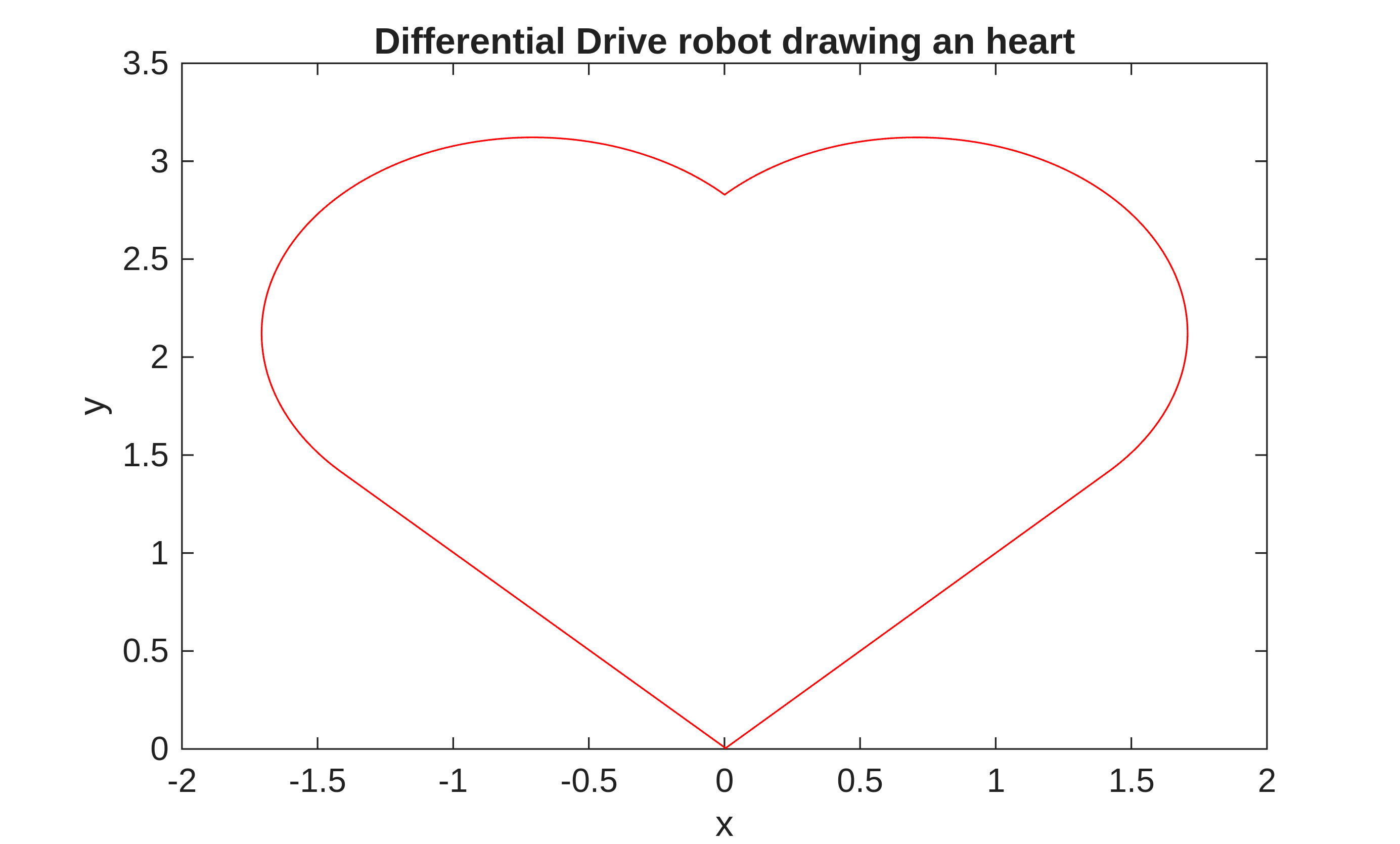
Using this model, a “drawer” function block calculates \(v\) and \(\omega\) starting from a trajectory,

then giving as an input to a Differential Drive Kinematic Model.
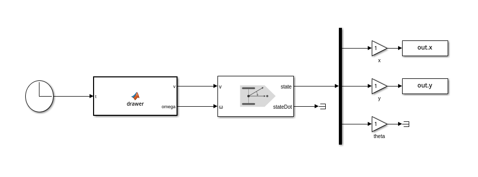
DiffDriveKinModel
 1
 2
 3
 4
 5
 6
 7
 8
 9
10
tsim=16;
stepsize=5e-3;
out=sim("model.slx");
x=out.x.data;
y=out.y.data;
figure(5)
plot(x,y,"red")
title("Differential Drive robot drawing an heart")
xlabel("x")
ylabel("y")
LoveYou妨